Pandas+Matplotlibで市町村の人口を可視化する
(Gistにipynbファイルをアップロードしています。ブログのレイアウトが読みにくい場合はこちらを御覧ください。)
今回は以下のような図をPythonで作ってみたいと思います。
試しに北海道の全人口(平成27年で538万3579人)が二等分されるように分けてみたんだが、たったこれだけでJR北海道が死にかけてる理由が察せるのが哀しい。 pic.twitter.com/z3EivEkvXM
— 道民の人@冬コミ廃墟本委託中 (@Tusk_act2) 2016年11月26日
シェープファイルを取り込む
地図のような境界や領域を保持しているファイルをシェープファイルといいます。シェープファイルの可視化はRでは結構情報が多いものの、Pythonだとなかなか活用例が少ない印象です。今回はこちらのサイトで配布されている平成25年度のシェープファイル及びその中の人口データを用いて、都道府県の人口を2分割するプログラムをPythonで書いてみました。 (たぶんもっとスマートな書き方があるような気がします…)
なお、Pythonでシェープファイルを扱うにはpyshpというモジュールをインストールする必要があります。
%matplotlib inline
from itertools import chain
import pandas as pd
import numpy as np
import shapefile
import matplotlib.pyplot as plt
from matplotlib.patches import Polygon
from matplotlib.collections import PatchCollection
import seaborn as sns
def list_to_dict(lst):
    return dict(zip(range(0, len(lst)), lst))

def list_flatten(lst):
    # 2重リストを1重にする
    return list(chain.from_iterable(lst))

def list_combine(lst, *args):
    for l in args:
        lst.extend(l)
    return tuple(lst)
# 点列と分割点のリストからPolygonのリストを作る
def make_polygons(row):
    row = row.tolist()
    axis = row[0]
    parts = list(row[1])
    parts.append(len(axis))
    axis_list = [axis[parts[i]:parts[i + 1]] for i in range(len(parts) - 1)]
    Polygons_list = [Polygon(x) for x in axis_list]
    return Polygons_list
# データの読み込み
sf = shapefile.Reader("japan_rvis_h25/japan_rvis_h25")
sf.shapes()[:10] # これら1つ1つがポリゴンデータ
[<shapefile._Shape at 0x108418cf8>,
 <shapefile._Shape at 0x108418f28>,
 <shapefile._Shape at 0x108418f60>,
 <shapefile._Shape at 0x108418b00>,
 <shapefile._Shape at 0x108418048>,
 <shapefile._Shape at 0x1084180f0>,
 <shapefile._Shape at 0x108418208>,
 <shapefile._Shape at 0x108418d68>,
 <shapefile._Shape at 0x1084182e8>,
 <shapefile._Shape at 0x108418390>]
データにはRecordとFieldが含まれており、前者はいわゆるポリゴンデータ、後者はその境界・領域についての属性データ(県名、市区町村名、人口など)になっています。
ポリゴンデータの中には市区町村の領域を結ぶための点列sf.shapes()[i].pointsがあるのですが、一部の市区町村は飛び地などによって境界が一筆書き出来ない地域があります。そのため、分割点のリストsf.shapes()[i].partsでそれらの点列をどこで分割するのかが明示されています。
field_name = [x[0] for x in sf.fields[1:]] # 属性データの項目
records = [[x.decode("shift-jis") if isinstance(x, bytes) else x for x in y]
                   for y in sf.iterRecords()]  #属性データのSHIFT-JISをデコード

sr_points = pd.Series(
    [i.shape.points for i in sf.shapeRecords()]).to_frame().rename(
        columns={0: "AXIS"})  # ポリゴンデータ
sr_parts = pd.Series([s.parts for s in sf.shapes()]).to_frame().rename(
    columns={0: "PARTS"})  # ポリゴンの分割点
field_name # 属性データの項目
['KEN', 'SICHO', 'GUN', 'SEIREI', 'SIKUCHOSON', 'JCODE', 'P_NUM', 'H_NUM']
# ポリゴンデータ(1行が1つの市区町村に対応)
sr_points.head(5)
AXIS
0
[(141.389636, 43.068598000000065), (141.387047...
1
[(141.405346, 43.18949900000007), (141.4073640...
2
[(141.4493920000001, 43.162633000000085), (141...
3
[(141.47346200000004, 43.096119000000044), (14...
4
[(141.43406900000002, 43.026091000000065), (14...
# 分割点のリスト
sr_parts.head(15)
PARTS
0
[0]
1
[0]
2
[0]
3
[0]
4
[0]
5
[0]
6
[0]
7
[0]
8
[0]
9
[0]
10
[0, 1549, 1553, 1557, 1562, 1567, 1571, 1576, ...
11
[0, 8, 13, 17, 21, 25, 29, 34, 1071, 1075, 107...
12
[0]
13
[0, 664, 675, 680, 686, 693, 700, 712, 716, 72...
14
[0, 1672, 2599, 2604, 2609, 2615, 2619, 2623, ...
Dataframeに統合
これらをPandasのDataframeとしてまとめます。この段階で点列と分割点のリストからMatplotlibのPolygonオブジェクトを作り、その列をDataframe内に作っておいてしまいます。(少し計算に時間がかかるかも)
# Dataframeでまとめる
df = pd.DataFrame(records).rename(
            columns = list_to_dict(field_name)
        )[["KEN", "SEIREI", "SIKUCHOSON","JCODE","P_NUM"]].assign(
            # 空白の数値データを0で埋める
            P_NUM = lambda df: df["P_NUM"].apply(lambda x: 0 if isinstance(x, str) else x),
        ).applymap(
            # 文字列のスペースを消去
            lambda x: x.strip() if isinstance(x, str) else x
        ).applymap(
            # 文字数ゼロをNaNにする
            lambda x: np.nan if x == "" else x
        ).join(
            # ポリゴンと分割点を統合
            [sr_points, sr_parts]
        ).assign(
            # MatplotlibのPolygonオブジェクトのインスタンスの列をつくる
            POLYGON = lambda df: df[["AXIS", "PARTS"]].apply(lambda x: make_polygons(x), axis=1)
        ).drop(
            # いらなくなったポリゴンと分割点を除去
            ["AXIS", "PARTS"], axis=1
        )
# データの確認。札幌市が区ごとに別のデータになっているのが分かる。
df.head(10)
KEN
SEIREI
SIKUCHOSON
JCODE
P_NUM
POLYGON
0
北海道
札幌市
中央区
01101
220189.0
[Poly((141.39, 43.0686) ...)]
1
北海道
札幌市
北区
01102
278781.0
[Poly((141.405, 43.1895) ...)]
2
北海道
札幌市
東区
01103
255873.0
[Poly((141.449, 43.1626) ...)]
3
北海道
札幌市
白石区
01104
204259.0
[Poly((141.473, 43.0961) ...)]
4
北海道
札幌市
豊平区
01105
212118.0
[Poly((141.434, 43.0261) ...)]
5
北海道
札幌市
南区
01106
146341.0
[Poly((141.164, 43.0851) ...)]
6
北海道
札幌市
西区
01107
211229.0
[Poly((141.328, 43.0861) ...)]
7
北海道
札幌市
厚別区
01108
128492.0
[Poly((141.473, 43.0961) ...)]
8
北海道
札幌市
手稲区
01109
139644.0
[Poly((141.283, 43.1336) ...)]
9
北海道
札幌市
清田区
01110
116619.0
[Poly((141.444, 43.0223) ...)]
政令指定都市は区としてバラバラの行として登録されています。今回はこれを統合して集計することにします。 (例:札幌市はそれぞれ北区、西区etc..として領域も人口もバラバラに登録されているが、これを札幌市1つとして統合)ちなみに東京の特別区(23区)は最初から市町村として入っているので、そのままになります。
# 政令指定都市一覧
df["SEIREI"].dropna().unique()
array(['札幌市', '仙台市', 'さいたま市', '千葉市', '横浜市', '川崎市', '相模原市', '新潟市', '静岡市',
       '浜松市', '名古屋市', '京都市', '大阪市', '堺市', '神戸市', '岡山市', '広島市', '北九州市',
       '福岡市', '熊本市'], dtype=object)
df_agg = df.drop(
                df.ix[df["SEIREI"].notnull()].index  # 政令指定都市である地域を削除
            ).append(
                # 政令指定都市を統合したデータを追加
                df.groupby(["KEN","SEIREI"]).agg(
                    {"P_NUM": np.sum ,
                     "POLYGON": list_combine,
                     "JCODE": lambda sr: sr.iloc[0]}
            ).reset_index().assign(
                # ポリゴンデータも統合
                POLYGON = lambda df: df["POLYGON"].apply(list).apply(list_flatten)
            )
        ).drop("SEIREI", axis=1).sort_values("JCODE").reset_index(drop=True)
# 札幌市をまとめた。(SIKUCHOSONがNaNになってしまってはいるが)
df_agg.head(10)
JCODE
KEN
POLYGON
P_NUM
SIKUCHOSON
0
01101
北海道
[Poly((141.39, 43.0686) ...), Poly((141.405, 4...
1913545.0
NaN
1
01202
北海道
[Poly((140.865, 42.0094) ...), Poly((140.935, ...
279127.0
函館市
2
01203
北海道
[Poly((141.01, 43.2417) ...), Poly((140.987, 4...
131928.0
小樽市
3
01204
北海道
[Poly((142.432, 43.9473) ...)]
347095.0
旭川市
4
01205
北海道
[Poly((140.99, 42.4373) ...), Poly((140.944, 4...
94535.0
室蘭市
5
01206
北海道
[Poly((144.222, 43.5211) ...), Poly((143.77, 4...
181169.0
釧路市
6
01207
北海道
[Poly((143.147, 42.9507) ...)]
168057.0
帯広市
7
01208
北海道
[Poly((143.776, 44.1847) ...)]
125689.0
北見市
8
01209
北海道
[Poly((142.279, 43.2253) ...)]
10922.0
夕張市
9
01210
北海道
[Poly((141.694, 43.3315) ...)]
90145.0
岩見沢市
人口で塗り分け
人口2分割を今回は冒頭の図と同じく北海道でやってみます。
なお、地域の分割の方法は単純に人口の多い市区町村から順に塗っていくものとします。
def make_majority_index(df):
    half_total_P_NUM = df.query("KEN == @prefecture")["P_NUM"].sum() / 2  # 県の人口の半分
    max_index = df.query("KEN == @prefecture")["P_NUM"].idxmax()  # 最大の人口を抱える市区町村のインデックス
    # 人口の多い地区を上から順番に、人口の半分を超えるまで選択する
    majority_index = df.query("KEN == @prefecture").sort_values(
        "P_NUM", ascending=False).assign(
            cum_P_NUM=lambda df: df["P_NUM"].cumsum()).query(
                "cum_P_NUM < @half_total_P_NUM").index
    if majority_index.size == 0:
        # 1つの地域だけで半分を超えた場合はその最大地域を採用
        majority_index = [max_index]
    return majority_index
prefecture = "北海道"
majority_index = make_majority_index(df_agg)  # 人口が多い方(分割で赤く塗る方)の市区町村のインデックスの列
# 県人口の半数を占める市町村
df_agg.query("index in @majority_index")
JCODE
KEN
POLYGON
P_NUM
SIKUCHOSON
0
01101
北海道
[Poly((141.39, 43.0686) ...), Poly((141.405, 4...
1913545.0
NaN
1
01202
北海道
[Poly((140.865, 42.0094) ...), Poly((140.935, ...
279127.0
函館市
3
01204
北海道
[Poly((142.432, 43.9473) ...)]
347095.0
旭川市
5
01206
北海道
[Poly((144.222, 43.5211) ...), Poly((143.77, 4...
181169.0
釧路市
# 上で選択したmajority_indexを用いてPolygonの塗り分けを選ぶ
Polygon_red = df_agg.query("index in @majority_index")["POLYGON"]
Polygon_blue = df_agg.query("KEN == @prefecture and not index in @majority_index")["POLYGON"]
# プロット
with sns.axes_style('white'):
    fig = plt.figure(figsize=(15,10))
    ax = fig.add_subplot(111)

    ax.add_collection(PatchCollection(list_flatten(Polygon_red.tolist()), facecolor="red", edgecolor='k', linewidths=.2))
    ax.add_collection(PatchCollection(list_flatten(Polygon_blue.tolist()), facecolor="blue", edgecolor='k', linewidths=.2))
    ax.tick_params(axis='x', which='both', top='off', bottom='off', labelbottom='off')
    ax.tick_params(axis='y', which='both', left='off', right='off', labelleft='off')
    ax.set_aspect('auto')
    ax.autoscale_view()
    plt.show()
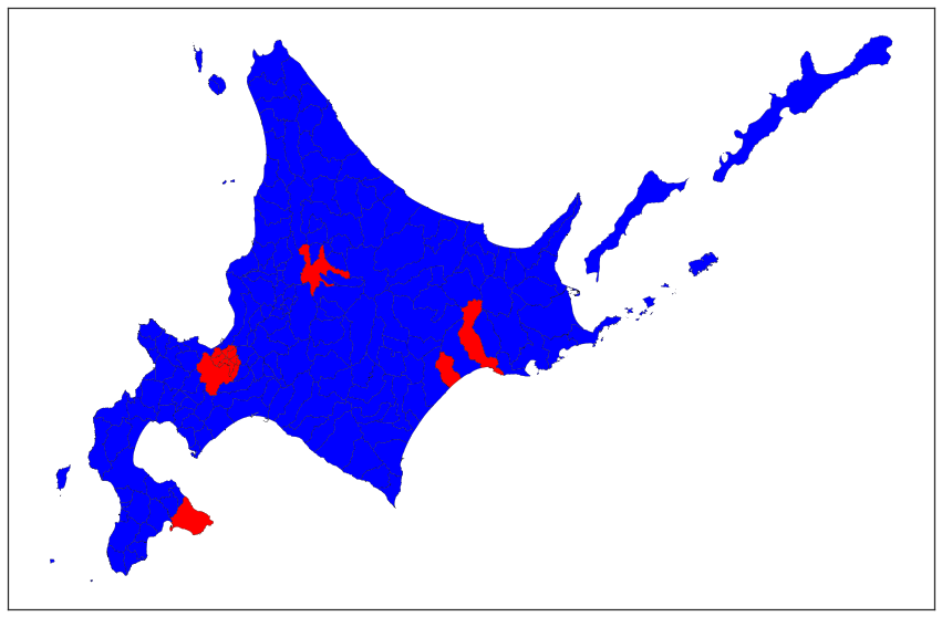
このように北海道の人口の偏りを可視化することができました。今回は単純に人口の多い市区町村から順に塗っていますが、札幌市の隣接地域から順番に塗っていくと冒頭のような図ができるのではないかと思います。